FCS Data Analysis Notes
Technical notes on analyzing fluorescence correlation spectroscopy data, divided into the following categories:
Technical notes on analyzing fluorescence correlation spectroscopy data, divided into the following categories:
FCS instruments provide a number of physically-relevant fitted parameters. These parameters are described below :
Correlation Time (τD) for one or more diffusing components
Average Number of Particles (Np)
Average Sample Intensity
Relative Concentration of Each Component
Counts per particle (CPP)
The QuantumXpert is optimized to characterize events that are relevant to biologists and biochemists -- specifically, the interactions of macromolecules (see Biological Interactions that FCS Can Detect). These events occur in the time domain of a few hundred microseconds up to a few seconds.
The QuantumXpert cannot be used to study fast photophysical events such as photon antibunching, triplet state dynamics, photoisomerization, or even rotational diffusion of molecules, all of which occur in the nanosecond to few microsecond time domain.
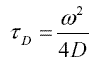
FCS data can report correlation time (τD) in both autocorrelation mode and cross-correlation mode. Correlation time is related to the translational diffusion coefficient, D, by the following relation:
where ω is the radius of the confocal detection volume.
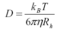
The diffusion coefficient of a particle is in turn determined by two properties: the viscosity of the solvent, η, and the hydrodynamic radius of the particle, Rh . This relationship is described by the Einstein equation :
where kB is the Boltzmann constant (1.38x10⁻²³ J/K) and T is the temperature.
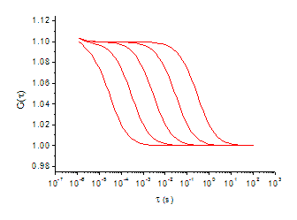
For autocorrelation experiments, where a single dye is measured in each emission channel, the magnitude of the change in molecular weight of free dye-labeled probe and probe-bound complex is critical, and will result in a right-ward shift in the correlation decay curve due to an increase in correlation time, as shown in Figure
A general rule-of-thumb is that the difference in molecular weight for the complex and the unbound probe should be between 3 to 5 fold to result in a shift in diffusion time that can be distinguished by FCS.
If two fluorescently labeled reactants are used, interaction between the two reactants can be monitored using cross-correlation and a large change in mass is not required. In this case, each fluorescent dye is detected in different emission channels, and the correlated diffusion between two channels result in the cross-correlation function.
FCS data also report the average number of fluorescently labeled particles (Np) in the detection volume. This value can be used to calculate the total concentration of the fluorescent particles in a sample.
Np is inversely proportional to the y-intercept, G(0), of the autocorrelation function, so as the average number of particles decreases, the magnitude of the intercept increases.
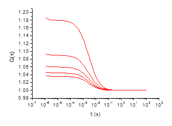
Figure: Shift in Particle Number (Np).
An interesting result of the inverse relationship between Np and the y-intercept is that the quality of FCS data can often be improved by reducing the concentration, rather than increasing the concentration. This is because a background FCS curve showing no correlation is centered at G = 1. Lowering the sample concentration will separate it further from baseline FCS curve because the intercept is higher (unless the signal intensity from the lower concentration sample becomes too faint).
FCS curves are created by correlating nanosecond fluctuations in fluorescence intensity. The steady-state average intensity can also provide useful information and is provided by most FCS instruments.
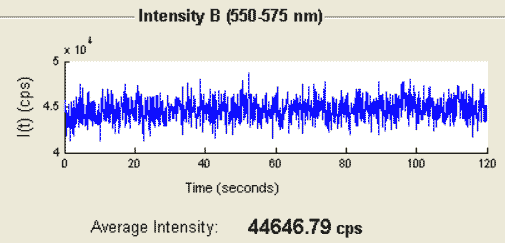
Figure: Average Intensity Trace.
In addition to reporting a value for Np, the average number of fluorescent particles, FCS data report the fraction of Np that is associated with components of different size. (Usually, components must differ in size by 3 to 5 fold to be distinguished.) These values can be used to calculate relative and absolute concentrations of each fluorescent species in a sample.
It is important to note that the contribution of each component to the correlation curve is related to both relative concentration and relative brightness. See Interpreting Fitted Fractions in FCS for information on how to take brightness into account when calculating relative concentrations.
The values of average intensity and number of particles can be used to calculate the average counts per particle to determine the degree of labeling of the fluorescent particles.
A "system response correction" for fluorescence correlation data taken on the QuantumXpert FCS spectrometer is built into the accompanying FCSXpert analysis software. The two parameters associated with this correction are A, the amplitude of this contribution, and τC, the fast time constant for this correction.
For a more detailed discussion, please see Autocorrelation Due to Other Phenomena in Mathematics of Autocorrelation.
When fitting experimental data to mathematical models, one often is confronted with the question of whether a more complicated model (e.g. one with more diffusion times) represents a “better fit.” Answering this question is a seven step process:.
It should be pointed out that the F-test does not enable us to compare different models with the same number of parameters and, therefore, the same degrees of freedom (e.g. one component diffusion with system response correction vs. two component diffusion without system response correction). Fundamentally, the F-test asks whether the addition of parameters statistically improves the fit.
The following examples will walk you through the process of applying the above model comparison procedure.
Below, we have provided an example of applying the above procedure to the process of fitting fluorescence correlation spectroscopy (FCS) data to two models: one component diffusion without system response correction and one component diffusion with system response correction.
The FCS model with the fewest parameters is that of one component diffusion:

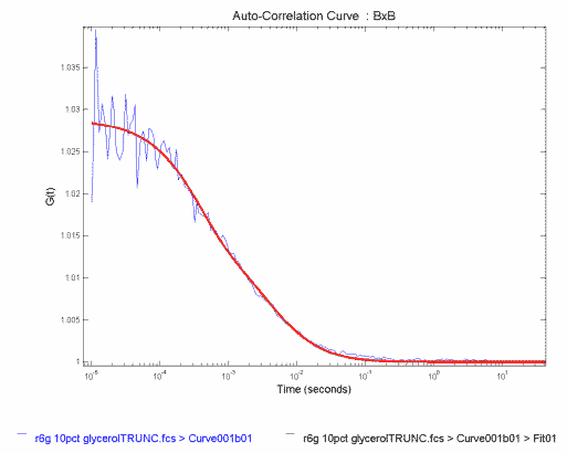
In Figure, we show a correlation function obtained for Rhodamine 6G in a 10% glycerol, 90% water solution (blue). The one-component fit to this correlation curve is shown in red.
Figure: FCS Correlation Data for Rhodamine 6G in Glyceral/Water fit to Single Component Diffusion
The results of the fit are
where Degrees of Freedom is equal to the number of data points - (number of parameters - 1), that is, 176-(2-1)=175, and SSE is the sum of the squares of the residuals.
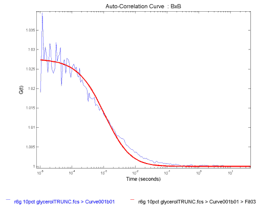
We look at the fit. It does a reasonable job of fitting the data in the beginning, then systematically over estimates the curve, and finally under estimates it. This is most clearly seen in the residuals (Figure 2), which are the differences between the data and the fitted curve. The residuals of a good fit fluctuate randomly and tightly about zero. In our data, we instead see large systematic variations, so we conclude that this model is not the best fit to our data and move on to Step 3.
Figure: Residuals of the Single Component Fit to the FCS Correlation Data in Figure 1
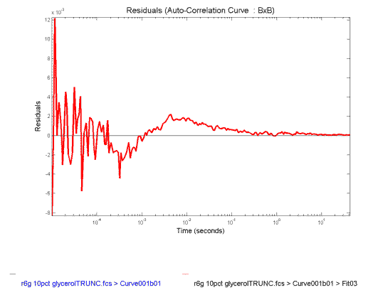
The net effect of the systematic variations in the one-component fit is that the obtained τD of 1.1 msec is faster than the value expected. We are expecting a number in excess of 3.0 msec because the beam radius is 1.8 um for the system used and the diffusion coefficient of Rhodamine 6G is ~2.8 cm2/sec. Because the results do not make physical sense, so we reject this fit and move on to Step 4.
We refit the data to the more complex model of one-component diffusion with system reponse:

The resulting fitted curve is shown in Figure,FCS Correlation Data for Rhodamine 6G in Glycerol/Water fit to Single Component Diffusion with System Response
The results of the fit are
where A is a system response correction factor and TauC is the correlation time of the system response.
The degrees of freedom are reduced by two because we have added the parameters τC and A.
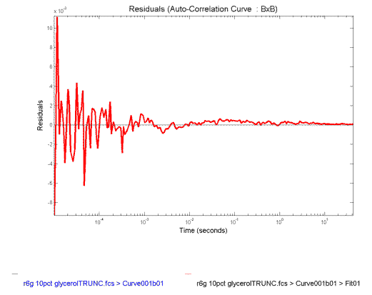
The residuals of the fit to the model of one-component with system response are shown in Figure
Figure 4: Residuals of the Single Component with System Response Fit to the FCS Correlation Data in Figure 3
The fit looks reasonable (Figure 3), except perhaps near the end. And this is confirmed by the fact that the residuals (Figure 4) are more tightly varying about zero.
We look at the fitted parameters. The τD of 3.3 ms is just what we are expecting from what we know of the physical characteristics of the sample, so we don't reject this fit yet.
We need, of course, to put our intuition on firm statistical grounds, so we perform an F-test to compare the two fits. The F-test asks the question: "What is the probability, p, that adding these two parameters improves the SSE by random chance?" We will set our threshold at < .05, or 5%, to consider the improvement real. One calculates the F-value with the following equation:
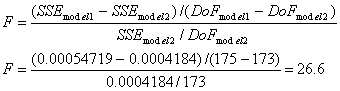
where we have used DoF to denote degrees of freedom and model 2 is the more complex model. Note that it is assumed that SSE for model two is smaller than SSE for model one. If not, F is negative and you have not improved the fit.
We can find the probability, p, associated with our F-value by consulting a table of F-values (see for instance F-value table) or using a calculator such as F-test Probability Calculator. To use these tools, we define the numerator degrees of freedom, DoFn to be DoF2 - DoF1 and the denominator degrees of freedom, DoFd to be DoF2. In general, the smaller the F-value is, the more likely it is that the improvement is due to random chance. This means that large F-values indicate a higher probability that the more complex model is correct..
In the present example, F = 26.6. Using a calculator, we see that for DoFn = 2, DoFd = 173, and F = 26.6, p < 1x10⁻¹⁰. We therefore conclude that the addition of parameters is justified and choose the more complex model. (Alternatively, we can look up the F-value corresponding to p = 0.05, F0.05, for our DoF values. Since our value of F = 26.6 is greater than F0.05 = 3.05, we can conclude that the more complex model is correct.)
There is a small but important issue to keep in mind when averaging data from FCS measurements. Consider Table 1, to the right. In the first column we list a set of correlation times,τ<sub>D</sub> obtained for a sample with an FCS instrument. In the second column we have calculated the diffusion coefficients (D) based on a beam radius of 1.5 µm and using the equation:

| τD (ms) | D x 10-8 cm2/sec |
|---|---|
| 76.37 | 7.37 |
| 77.27 | 7.28 |
| 62.73 | 8.97 |
| 89.53 | 6.28 |
| 144.5 | 3.89 |
| 101.9 | 5.52 |
| 62.99 | 8.93 |
| 162.7 | 3.46 |
| 122.5 | 4.59 |
| 154.8 | 3.63 |
If we average the column of correlation times we obtain (106 ± 38) ms. If we use this average correlation time to calculate an average diffusion coefficient, we obtain (5.4 ± 1.9) x 10-8 cm2/s. If we instead average the column of diffusion coefficients, we obtain D = (6.0 ± 2.1) x 10-8 cm2/s. The diffusion coefficient obtained from averaging the diffusion coefficients is 11% higher than that obtained from the average correlation time. This is because averaging correlation times favors large times, while averaging diffusion coefficients favors short times.
Which is the correct number to report? Here is the bad part, both are acceptable. What is important is that you specify how your measurements were done, and that, if you are comparing your results to someone else's, you need to know how they obtained their averages.
In Autocorrelation Due to Multicomponent Translational Diffusion we derived the FCS equations for multicomponent diffusion as follows:

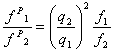
One caveat to the general equation for multicomponent diffusion is that the counts/particle of all components is assumed to be the same. At the end of Autocorrelation Due to Multicomponent Translational Diffusion, we derived an equation for converting fractions resulting from fitting to the above equation, f1 and f2, to the physical particle number fractions, fP1and fP2 as follows:
where q1 and q2 are counts/particle for component 1 and 2, respectively.
A Sample of Monomers & Known Oligomers: Calculating fP1 and fP2
In this example we will consider the case of a fluorescent molecule, such as a fluorophore-labeled protein, that exists as an equilibrium of two forms in solution: monomeric and oligomeric. We will calculate the relative and absolute concentrations of each component from fitted FCS results.In this example, the degree of oligomerization is known, and we will use the example of tetramerization.
This analysis might be used to determine the affect of environmental factors, such as pH or temperature, on the relative equilibrium monomer/oligomer concentrations.
An autocorrelation curve of the sample above will have two diffusing components. A fit to the autocorrelation curve will output these parameters:
where component 2 is the larger, slower-diffusing component.For this example, we will use the following representative results:
and assume that the oligomer is a tetramer made up of four monomeric units, which means that q2 = 4q1 (assuming that no change in fluorophore quantum yield is observed upon tetramerization). We will also use a confocal instrument detection volum e of 20 fL (20x10-15 L), which means that a particle number of Np = 50 corresponds to 4.2 nM.
Because f1 and f2 aren't the physical fractions of particle number, we need to apply the correction equation to find the equilibrium concentrations of each component.
Using the following equation,
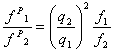
we can calculate fP1 / fP2 = 5.33.
Using the condition that fP1 + fP2 = 1, we find that:
where we have corrected for the overestimation of component 2's fraction due to the 4x increase in brightness and we see that component 1 is actually the dominant component.
Finally, If we use the total conentration of 4.2 nM, we can calculate that the concentration of each component as: